Linear Prediction of Speech
The originators of the technique, Bishnu Atal and colleagues, were working
on television pictures, two dimensional images changing in time. One way of
representing such an image is as a two dimensional matrix of numbers, each
representing the brightness of one spot on the screen, each pixel. The representation
of a single image would require a very large matrix of numbers, and to represent
a changing sequence of images, many images per second, would require huge
quantities of data. However that approach overlooks a fact about images:
the brightness of any particular point is not independent of the brightness
of neighbouring points in the image, because on a television image there
are regions of light and dark and different shades in between. A pixel doesn’t
vary too much from the brightness of its neighbours. In other words there
is a strong correlation between the brightness of any given pixel and the
brightness of its neighbours. The same holds true for speech signals, as
we can see in figure 5.5.
Figure 5.5. Portion of a signal modelled by regression
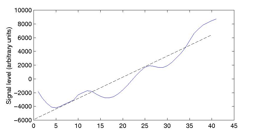
Sample number
There is a strong correlation between the magnitude of a signal at any given
sample and the magnitude of the immediately preceding samples. The magnitude
of the signal at each sample is often predictable by considering the magnitude
of the signal for the preceding few samples. Of course if we predict the value
of the magnitude of the signal at one point in time on the basis of linear
regression from the preceding samples, the actual magnitude of the signal
in that sample might be something different from our prediction. The prediction
could be in error one way or the other, too high or too low. In figure 5.5,
for example, the equation of the linear regression line (dashed) is x
[t] = 308.35 t – 5928.8, so for the next point, t =
41, we predict that x[t] will be 6714. In fact, the actual
value is 8738. However if we take the difference between the predicted value
and the actual value, the size of the difference between the prediction and
the actual value is in general very much less than the magnitude of the signal
itself at that point. In this case, the difference is –2024, an underestimate.
As we go through the signal making predictions as to what the next value of
the signal is going to be based upon the previous handful of samples, our
prediction will be more or less in error. But if we store the errors as a
separate signal the combination of the predicted signal (according to the
predictor coefficients) and the stored error accurately encodes the original
signal. The amount of information that we need to store can be significantly
less than simply storing the value of each successive sample.
Next: Linear Prediction
equation