The mathematics of the relationship between prediction
coefficients and formant frequencies and bandwidths is too complex to cover
in this course. But the method is very simple. Consider a single frame of
linear prediction coefficients, for instance, 10 coefficients relating to
the 80-sample frame around sample 8000 of joe8k.dat. (That frame falls in
the middle of the [a] of “father”.) Those coefficients are plotted
in figure 5.7.

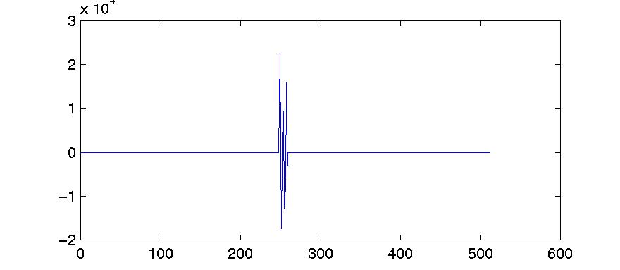
We beef these numbers up (by multiplying them by 15,000) and add zeroes at the start and end, to make a signal portion 512 samples long, as in figure 5.8.
Figure 5.7. Ten LPC coefficients from [a] in
joe8k.dat
LP coefficient
number
We beef these numbers up (by multiplying them by 15,000) and add zeroes at the start and end, to make a signal portion 512 samples long, as in figure 5.8.
Figure 5.8. The same ten LPC coefficients scaled up
and zero-padded to 512 samples
Sample Number
The Fourier transform of this brief, blip-like signal has a very smooth spectrum, as figure 5.9 illustrates. It has amplitude peaks at 343–390 Hz (i.e. centred on 356 Hz), 2656 Hz, and 3656 Hz. Those figures are the first, second and third formants of the vowel. Because it is so easy to measure formants in this way, linear prediction has become the standard method of automatic formant tracking.
Figure 5.9. LPC spectrum of [a]
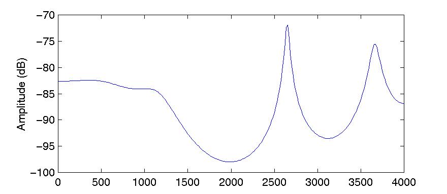
Frequency (Hz)
Frequency (Hz)
A program that implements this method is provided in
lpc_spectrum.c
. I shall not give a listing or discuss its operation in detail here,
as it merely puts together techniques we have seen already: the explanation
above must suffice. When compiling it, it must be linked with nrutil.o
and memcof.o, as we saw with lpcana.c, above. When compiled,
lpc_spectrum takes two arguments: a signal file name and the sample
number of interest, and outputs the spectrum as text to standard output.
Figure 5.9 was plotted from the output of lpc_spectrum.