Example of linear prediction of speech

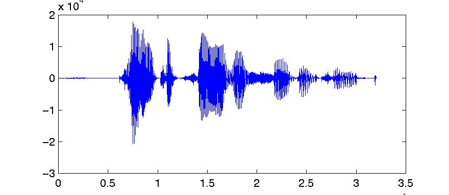
A comparison between joe.dat and joe_err.dat is given in figure 5.6.

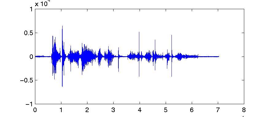
b) First 32000 samples of joe_err.dat

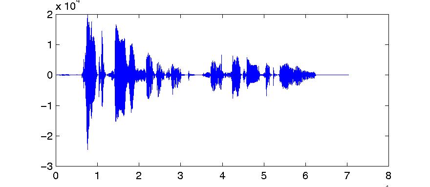
c) First 32000 samples of joe_lpc.dat

Note that the residual, in figure 5.6 (b), is a lower-amplitude signal than the original. The prediction residual has sharp spikes at regular intervals, corresponding to the glottal pulses of the speech wave. Those spikes occur in the prediction residual at those points in the speech wave at which the signal is changing direction in a very extreme fashion. At those points, the linear prediction idea does not work very well, and we get a big error. As the spacing of those spikes occurs at the fundamental frequency of the original speech, the occurrence of a spike in the prediction residual is again highly correlated with the location of spikes on previous cycles. So by estimating the pitch, we could remove (or at least reduce) the spikes from the prediction residual. Practically all that is left in the prediction residual after pitch prediction is just residual noise.

Next: Linear prediction analysis